

This course complements the previous training on camera trapping methods and protocols, specifically the random encounter method (REM).
Introduction to the 3rd online training course
by Joaquín Vicente
Tips for improving distance data digitalization on AGOUTI
by Marcus Rowcliffe
- Digitise deployment pole and animal positions in Agouti. The mechanics of this have already been covered, but some important points to note when digitising poles:
- Double check pole heights
- Be careful if you can’t be sure that the pole is resting on the ground.
And some points to note when digitising animal observations:
- Digitise animal positions on the ground – this is often further down the image than you think.
- Keep an eye on the time stamp to ensure that multiple observations within sequences are separated. An observation should have gaps between images of no more than a few seconds.
When finished digitising, export the project and extract the resulting zip file in an appropriate location (you may find that the downloading indicator continues to spin after the download complete – try refreshing the browser page occasionally).
R-analysis tool: and interface to estimate density (REM) on standardized exports.
by Marcus Rowcliffe
Instructions
If you don’t already have them, install:
R: https://cran.r-project.org/
RStudio: https://posit.co/download/rstudio-desktop/
Download example files:
Example data package and Code and documentation
Move the resulting zip file from your downloads folder to a more memorable location and rename it if preferred, then extract it.
You should find two things in the resulting folder:
A folder called data; this is an example data package as produced by an Agouti export.
A file called rem_example.R; this contains R code for running an example REM density analysis.
Open RStudio and set up a new project
- File > New Project > Existing Directory > Browse to the folder you just extracted from the Github download > Create Project.
- In the lower right RStudio panel you should see a tab called Files – click on this (if not already highlighted) and you will see your project files. Click on rem_example.R.
- Before you can start analysing, you will need to install some additional packages as one-off. These will then be available in future analysis sessions without having to reinstall. Running the first chunk of code does this installation. To run a line of code, place the cursor on it and press Ctrl+Enter (Win) or Cmd+Enter (Mac).
Start analysing
- At start of each session, load the necessary libraries (run the second chunk of code).
- Load the data using the function read_camtrap_dp2. Note: this is a slightly modified version of the camtraptor function read_camtrap_dp which currently isn’t working properly with Agouti output. Once these internal data processing issues are fixed I’ll update the example and notify you.
- As a reminder, REM analysis requires component estimates to arrive at animal density:
- effective detection zone radius
- effective detection zone anglea
- verage speed while active
- proportion of time spent active
- trap rate (derived from numbers of independent contacts and effort at each camera location)
The analysis process requires a model to be fitted for each of the parameters.
The code sets out two possible ways of running an REM density estimation model:
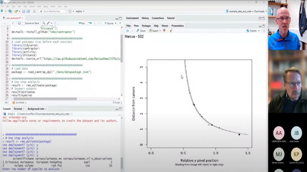
- A one-step process that only requires a datapackage as input. By default, this first asks you to check all the deployment diagnostic plots and say which species you want to analyse before running the analysis. Diagnostic plots should show reasonably good fits between trend line and data points. Very poorly fitting models should be marked for exclusion so that the unreliable animal position data from these deployments can be excluded from detection zone and speed models. The output of this function is a list with several components, accessed by typing a $ after the object name. For example, if you assigned the output to an object called result, you would find the following components:
result$estimates: a table of density and component parameter estimates, their standard errors, coefficients of variation, sample sizes and units.
result$species: the name of the species to which the results apply.
results$data: a table of the observation count and camera effort at each location.
result$speed_model, result$activity_model, result$radius_model, result$angle_model: these are the component parameter models, which can be inspected in various ways to check for reliability. Because they are fitted internally they have less flexibility in the modelling options, but the default options used are likely to be sensible and consistent in most cases. - A step-by-step approach in which you fit your own component models, allowing more flexibility if you believe it is necessary and are confident with the methods. I will take you through this process in the live session.
